
The Ultimate Guide to Development, Programming, Debugging and Verification
✔ New UMAT development ✔ Existing UMAT debugging
Whether you want to learn Abaqus UMAT, implement a constitutive model from a research paper, or need professional assistance to develop, debug, verify, or optimise a user material, this guide provides both technical knowledge and practical engineering solutions.
Abaqus UMAT (User Material Subroutine)
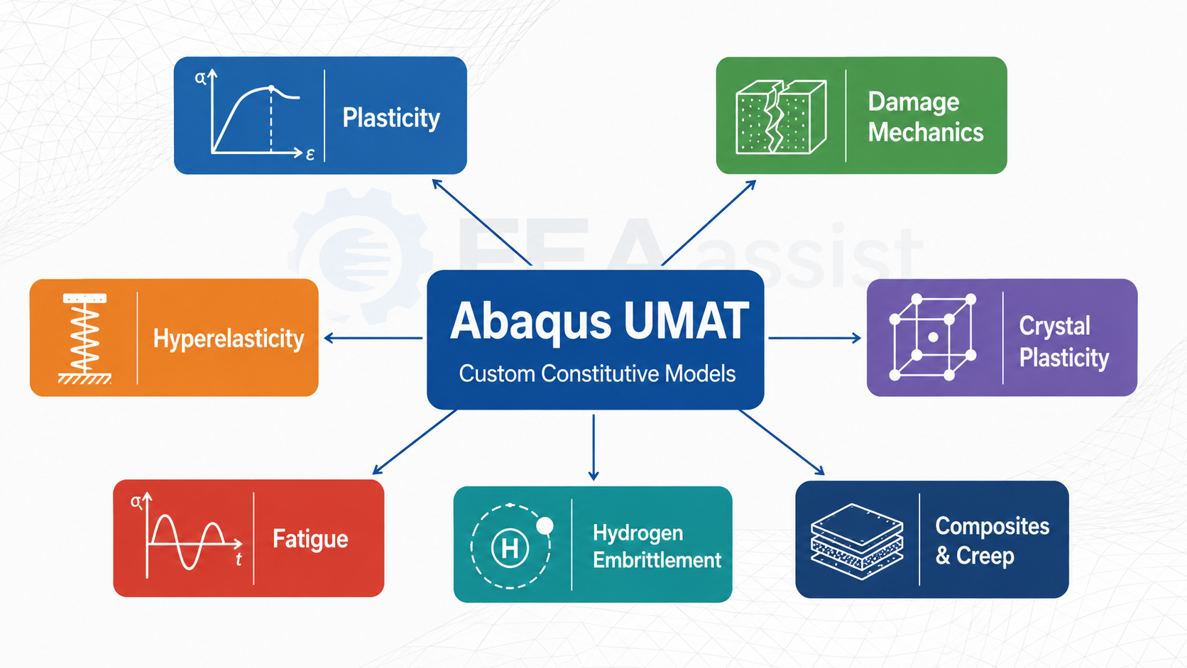
Abaqus UMAT (User MATerial Subroutine) is the primary user subroutine in Abaqus/Standard for implementing custom constitutive material models that cannot be represented using the built-in Abaqus material library. By writing a Fortran-based UMAT, researchers and engineers can define the complete mechanical behaviour of advanced materials, including nonlinear plasticity [1,2] damage [1], hyperelasticity, crystal plasticity [1,2,3,4], fatigue [1], hydrogen embrittlement [1,2,3], Composites [1,2,,3,4,5], Peridynamics [1], Phase field, [1], and many other complex constitutive models.
Why This Abaqus UMAT Guide Is Different
Developing a successful Abaqus UMAT is not simply a programming task. Many tutorials explain how to write a UMAT, but a robust implementation requires much more. The constitutive equations, DDSDDE (consistent tangent matrix), stress update algorithm, and state variables must all be implemented and verified correctly to achieve accurate and stable simulations.
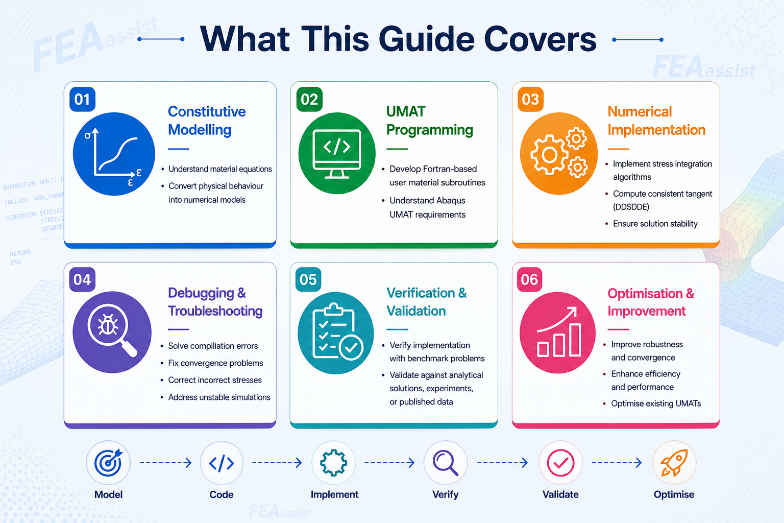
Unlike many online tutorials that focus mainly on Fortran syntax, this guide combines constitutive modelling, finite element theory, numerical algorithms, programming, debugging, verification, validation, and practical engineering experience [1,2] to explain how reliable UMAT implementations are developed.
Who Should Read This Guide?
This guide is written for anyone who needs to understand or work with Abaqus UMAT.
- 🎓 Students learning user material subroutines for the first time.
- 🔬 MSc and PhD researchers implementing constitutive models from scientific literature.
- ⚙ Simulation engineers developing advanced material models for engineering applications.
- 🏫 Universities and research groups validating numerical implementations.
- 🏭 Engineering companies requiring custom material model development.
- 🛠 Abaqus users facing UMAT errors, convergence problems, incorrect results, or debugging challenges.
Why Was UMAT Developed?
The behaviour of a material is governed by constitutive equations that describe how stresses evolve when a material experiences deformation. These equations can become extremely complex when considering nonlinear phenomena such as plastic deformation, damage evolution, anisotropy, rate dependency, phase transformation, or coupled physical processes.
Although Abaqus provides a large library of material models, advanced research and industrial applications frequently require models that are not directly available. UMAT provides the flexibility to implement almost any mechanical constitutive formulation by allowing the user to define the material response at each integration point during the analysis
How Does UMAT Work Inside Abaqus?
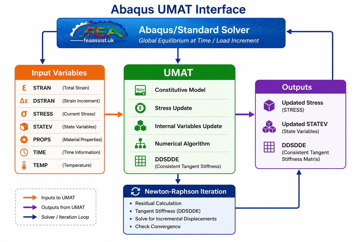
During an Abaqus/Standard analysis, the finite element solver divides the model into elements and evaluates the material response at integration points inside those elements. When a material definition uses UMAT, Abaqus automatically calls the user subroutine during the solution process.
At each increment, Abaqus provides the UMAT with the current material information, including deformation increment, previous stress state, material properties, and internal variables. The UMAT then calculates the updated stress state, updates state variables, and returns the material Jacobian matrix (DDSDDE) to the solver.
Unlike built-in Abaqus material models, UMAT allows users to define their own constitutive equations and numerical stress-update algorithms. Abaqus remains responsible for the global finite element solution, while UMAT provides the local material response at each integration point.
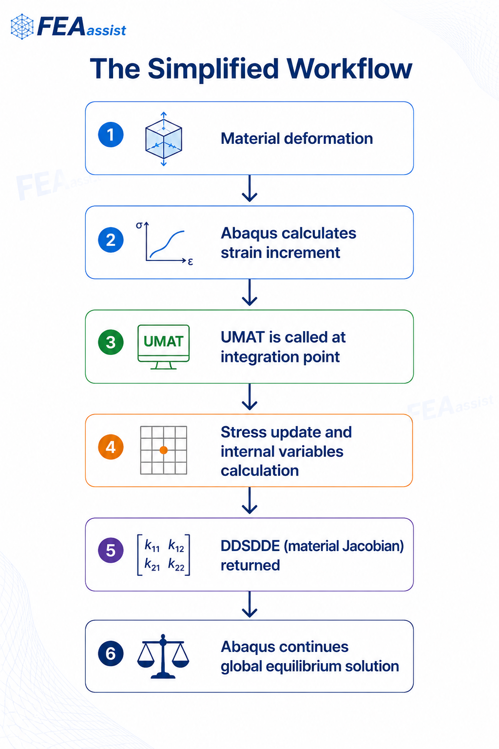
Understanding how Abaqus communicates with UMAT is one of the most important steps in learning user material subroutines. Many beginners focus mainly on Fortran programming without understanding when UMAT is called, what information is exchanged, and what results must be returned to Abaqus.
During each increment, Abaqus calls UMAT at every integration point where the user material is defined. The subroutine receives the current material state and performs the constitutive calculations required for that increment.
The main quantities exchanged between Abaqus and UMAT are:
- STRESS: Current and updated stress tensor
- STATEV: History-dependent internal variables
- DSTRAN: Strain increment for the current step
- PROPS: User-defined material parameters
- DDSDDE: Consistent material Jacobian matrix
After UMAT returns the updated stress, state variables, and DDSDDE matrix, Abaqus continues solving the global equilibrium equations using the Newton-Raphson iteration procedure.
UMAT Is More Than Writing Fortran Code
A common misunderstanding is that developing a UMAT is mainly a programming task. In reality, the Fortran code is only the final translation of a much larger engineering process.
A reliable UMAT requires several interconnected steps:
- Material theory: Understanding the physical behaviour and constitutive equations.
- Mathematical formulation: Converting the theory into stress update equations and internal variables.
- Numerical algorithm: Selecting appropriate integration methods and ensuring stability.
- Programming implementation: Writing the Fortran UMAT and connecting it with Abaqus.
- Verification: Checking the implementation using simple benchmark problems.
- Validation: Comparing simulation results against experiments or trusted references.
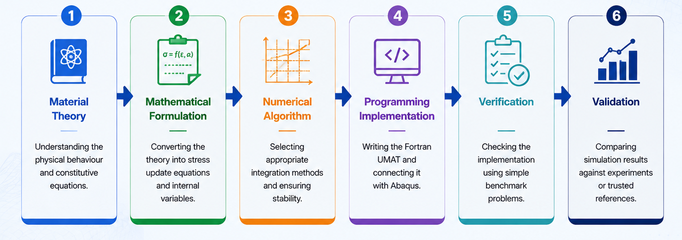
UMAT Is More Than Writing Fortran Code
A common misunderstanding is that developing a UMAT is mainly a programming task. In reality, the Fortran code is only the final translation of a much larger engineering process.
A reliable UMAT requires several interconnected steps:
- Material theory: Understanding the physical behaviour and constitutive equations.
- Mathematical formulation: Converting the theory into stress update equations and internal variables.
- Numerical algorithm: Selecting appropriate integration methods and ensuring stability.
- Programming implementation: Writing the Fortran UMAT and connecting it with Abaqus.
- Verification: Checking the implementation using simple benchmark problems.
- Validation: Comparing simulation results against experiments or trusted references.
Why Use Abaqus UMAT Instead of Built-In Material Models?
One of the most common questions asked by engineers and researchers is “Why should I write a UMAT when Abaqus already provides many built-in material models?”
The answer depends on the complexity of the material behaviour you need to simulate. Abaqus contains an extensive library of material models covering elasticity, plasticity, hyperelasticity, viscoelasticity, creep, damage, and many other engineering applications. For most conventional simulations, these built-in models are sufficient and require no programming.
However, research and industrial applications frequently involve constitutive equations that cannot be represented using the standard Abaqus material library. In these situations, Abaqus UMAT provides complete freedom to implement your own constitutive equations, stress integration algorithms, internal variables, and material Jacobian matrix (DDSDDE), allowing virtually any mechanical material model to be incorporated into Abaqus/Standard.
Typical Reasons for Using UMAT
- ✔ Implement constitutive models published in scientific journals.
- ✔ Develop new material models for MSc, PhD, or industrial research.
- ✔ Simulate advanced nonlinear material behaviour unavailable in Abaqus.
- ✔ Model coupled phenomena such as hydrogen embrittlement, fatigue, damage evolution, or crystal plasticity.
- ✔ Improve or extend an existing UMAT implementation.
- ✔ Optimise numerical stability and convergence behaviour.
- ✔ Validate new constitutive theories before publication or industrial application.
Need Help with Your UMAT?
Whether you need to learn Abaqus UMAT, develop a new constitutive model, debug an existing UMAT, or improve and optimise your implementation, FEAassist provides both comprehensive tutorials and professional engineering services.
How Abaqus UMAT Works Inside Abaqus/Standard
Understanding how Abaqus communicates with a UMAT is one of the most important steps in learning user material subroutines. Many beginners focus on writing Fortran code without fully understanding when the UMAT is called, what information Abaqus provides, and what the subroutine must return to the solver.
During every increment of an Abaqus/Standard analysis, the finite element solver evaluates the material behaviour at every integration point inside every element. If the material definition uses a UMAT, Abaqus temporarily transfers control to the user subroutine so that the material response can be calculated using the user’s constitutive model.
Instead of using one of the built-in Abaqus material models, the solver waits for the UMAT to calculate the updated stresses, update the material state variables, and return the material Jacobian matrix (DDSDDE). Once these values are returned, Abaqus continues solving the global equilibrium equations using the Newton-Raphson iteration procedure.
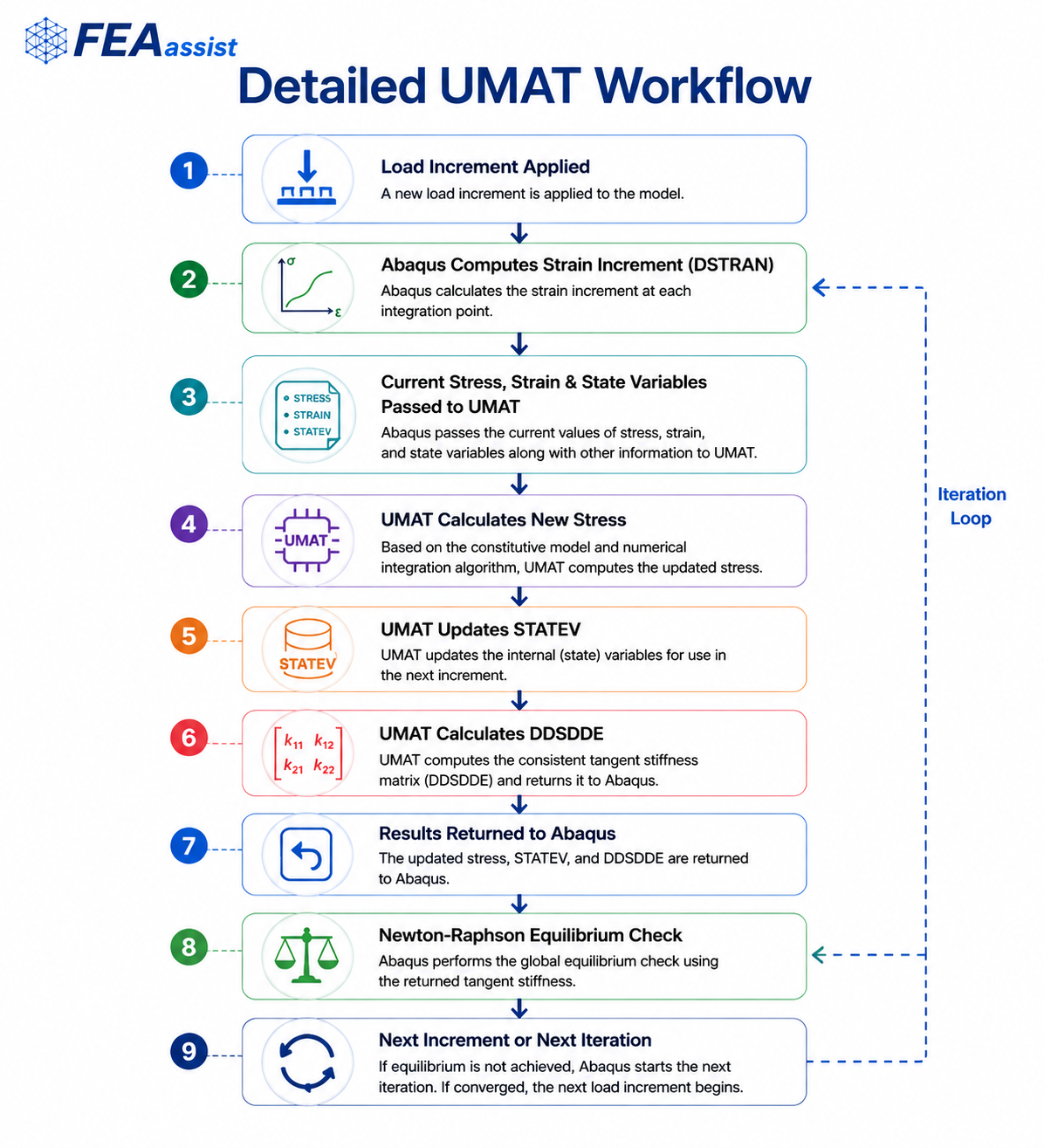
Simplified UMAT Workflow
Load Increment Applied
⬇
Abaqus Computes Strain Increment (DSTRAN)
⬇
Current Stress, Strain & State Variables Passed to UMAT
⬇
UMAT Calculates New Stress
⬇
UMAT Updates STATEV
⬇
UMAT Calculates DDSDDE
⬇
Results Returned to Abaqus
⬇
Newton-Raphson Equilibrium Check
⬇
Next Increment or Next Iteration
Information Passed from Abaqus to UMAT
Every time Abaqus calls the UMAT, it provides all the information required to compute the material response at the current integration point. These variables describe the current loading state, deformation history, material properties, and analysis conditions.
| Variable | Purpose |
|---|---|
| STRESS | Current stress tensor before updating |
| STRAN | Current total strain |
| DSTRAN | Strain increment for the current step |
| STATEV | Internal state variables such as plastic strain, damage variables or hardening parameters |
| PROPS | Material constants defined by the user |
| TIME | Current analysis time |
| TEMP | Current temperature if temperature-dependent behaviour is considered |
What Must the UMAT Return?
After performing the constitutive calculations, the UMAT returns several quantities that Abaqus requires to continue the finite element solution. These outputs determine both the material response and the convergence behaviour of the global analysis.
- Updated stress tensor (STRESS)
- Updated internal variables (STATEV)
- Consistent material Jacobian matrix (DDSDDE)
- Optional energy quantities
- Optional temperature-related variables
Among these outputs, the DDSDDE matrix is often the most critical. An inaccurate Jacobian matrix may still produce correct stresses, but it can significantly reduce convergence speed or even prevent the simulation from converging. This is why developing a reliable UMAT requires much more than simply writing Fortran code.
Professional UMAT Development
Understanding the UMAT interface is only the first step. Successfully implementing a constitutive model also requires selecting an appropriate stress integration algorithm, deriving the consistent tangent matrix, verifying the numerical implementation, and validating the results against experiments or reference solutions.
If you need assistance with developing a new UMAT, debugging an existing implementation, or improving convergence and numerical robustness, FEAassist provides professional UMAT development and consulting services.
Understanding the Abaqus UMAT Interface
One of the biggest challenges for new UMAT developers is understanding the large number of variables passed to the user subroutine. When Abaqus calls UMAT, dozens of arguments are supplied, each containing information about the current material state, loading conditions, geometry, analysis step, and material properties.
Although the complete UMAT interface may initially appear complicated, most constitutive models rely on a relatively small group of essential variables. Understanding these variables is far more important than memorising the complete subroutine declaration.
Whether you are learning Abaqus UMAT, implementing a constitutive model from a research paper, or developing a commercial material model, mastering the UMAT interface is the foundation of every successful implementation.
The Most Important UMAT Variables
| Variable | Purpose | Updated by UMAT? |
|---|---|---|
| STRESS | Current stress tensor | ✔ Yes |
| STATEV | Internal state variables | ✔ Yes |
| DDSDDE | Consistent material Jacobian | ✔ Yes |
| STRAN | Total strain | No |
| DSTRAN | Current strain increment | No |
| PROPS | Material constants | No |
| TIME | Current analysis time | No |
| PNEWDT | Suggest time increment adjustment | Optional |
Key Variables Explained
STRESS
The STRESS array contains the stress components at the current integration point. After performing the constitutive calculations, the UMAT must overwrite this array with the updated stresses corresponding to the new strain increment. Every material model ultimately exists to calculate these updated stresses accurately.
STATEV
STATEV stores the history-dependent variables required by the constitutive model. Typical examples include accumulated plastic strain, hardening variables, damage parameters, back stresses, phase fractions, or any other internal variables describing the material state. Because these variables are preserved between increments, they allow UMAT to model irreversible material behaviour.
DDSDDE
The DDSDDE matrix represents the consistent material Jacobian, often referred to as the tangent stiffness matrix. Although stress calculations determine the physical material response, DDSDDE largely controls the convergence behaviour of the Newton-Raphson solver. An inaccurate Jacobian frequently results in slow convergence, excessive iterations, or complete divergence even when the stress update itself is correct.
STRAN and DSTRAN
STRAN contains the total strain at the current increment, whereas DSTRAN contains only the strain increment applied during the current solution step. Most constitutive integration algorithms use DSTRAN to compute the stress increment while STRAN provides the accumulated deformation history.
PROPS
The PROPS array stores all material parameters entered by the user within the Abaqus material definition. These parameters may include elastic constants, yield stresses, hardening coefficients, damage parameters, viscosity constants, or any other material properties required by the constitutive equations.
PNEWDT
PNEWDT allows the UMAT to recommend increasing or reducing the time increment. Advanced constitutive models frequently use this variable to improve numerical stability during severe nonlinear behaviour, large plastic deformation, or damage evolution.
Practical Tip
Many beginners believe that writing a UMAT mainly involves programming. In reality, most development time is spent deriving constitutive equations, selecting an appropriate stress integration algorithm, managing internal variables, and ensuring that the returned DDSDDE matrix is mathematically consistent with the stress update. The Fortran implementation is only the final step of a much larger engineering workflow.
How Stress Integration Works in Abaqus UMAT
Once the UMAT receives the current material state from Abaqus, its primary responsibility is to calculate the material response for the applied strain increment. This process is known as constitutive integration or stress integration, and it is the core of every user material implementation.
The constitutive integration algorithm determines how stresses and internal variables evolve as deformation progresses. Depending on the constitutive model, this may involve simple elastic calculations or highly nonlinear iterative procedures for plasticity, damage mechanics, crystal plasticity, viscoplasticity, or coupled multi-physics problems.
Although the mathematical formulation differs between material models, almost every UMAT follows the same general workflow.
Typical UMAT Stress Update Workflow
Read material properties (PROPS)
⬇
Read previous stress (STRESS)
⬇
Read internal variables (STATEV)
⬇
Read strain increment (DSTRAN)
⬇
Compute trial (elastic predictor) stress
⬇
Check constitutive model or yield condition
⬇
Perform stress integration algorithm
⬇
Update stress tensor
⬇
Update STATEV variables
⬇
Compute DDSDDE
⬇
Return results to Abaqus
The Elastic Predictor Step
Many constitutive models begin by assuming that the entire strain increment behaves elastically. This temporary solution is called the elastic predictor or trial stress. The trial stress provides an initial estimate of the material response before checking whether the constitutive model allows purely elastic behaviour.
For linear elasticity, the trial stress immediately becomes the final stress. However, nonlinear constitutive models usually require additional calculations because the trial stress may violate the material’s yield surface, damage criterion, or other constitutive constraints.
Return Mapping Algorithms
For plasticity models, the trial stress often lies outside the admissible yield surface. In this situation, the stress must be projected back onto the yield surface using a return mapping algorithm. This procedure ensures that the updated stress satisfies the constitutive equations while maintaining numerical stability.
Return mapping algorithms are among the most widely used numerical techniques in computational plasticity and are commonly implemented in UMATs for isotropic plasticity, kinematic hardening, combined hardening, crystal plasticity, and many advanced constitutive formulations.
Updating the Internal Variables
Once the stress has been determined, the UMAT updates the STATEV array. These state variables preserve the loading history of the material and allow irreversible phenomena such as plastic deformation, damage evolution, hardening, creep, or phase transformation to accumulate throughout the analysis.
The number and meaning of STATEV variables depend entirely on the constitutive model. Simple elastic materials may not require any state variables, whereas advanced research models may store dozens of history-dependent quantities.
Computing the Consistent Tangent Matrix (DDSDDE)
After updating the stresses and state variables, the UMAT computes the consistent material Jacobian matrix (DDSDDE). This matrix describes how stress changes with strain and is essential for the Newton-Raphson solution procedure used by Abaqus/Standard.
Although Abaqus may still converge when an approximate tangent matrix is supplied, an inconsistent DDSDDE often leads to slow convergence, excessive equilibrium iterations, or divergence. Consequently, deriving the correct Jacobian is one of the most challenging aspects of UMAT development.
Engineering Insight
Many beginners believe that writing a UMAT mainly involves programming in Fortran. In practice, the programming itself is usually straightforward. The real challenge lies in developing a mathematically consistent constitutive model, selecting an appropriate stress integration algorithm, deriving the tangent stiffness matrix, and verifying that the implementation produces physically meaningful and numerically stable results.
If you need assistance with developing a new UMAT, debugging convergence problems, or improving an existing implementation, FEAassist provides professional consulting as well as a comprehensive Abaqus UMAT tutorial covering the complete development process.
How to Write an Abaqus UMAT Subroutine
Writing an Abaqus UMAT involves much more than programming in Fortran. Before writing a single line of code, the constitutive model must be clearly defined, the governing equations must be derived, and a suitable numerical integration algorithm must be selected. Only then can the mathematical model be translated into a reliable and efficient UMAT implementation.
A successful UMAT is therefore the combination of material science, continuum mechanics, numerical methods, finite element analysis, and programming. The Fortran source code simply connects these engineering concepts to the Abaqus solver.
Whether you are implementing a constitutive model from a scientific publication or developing a completely new material formulation, nearly every UMAT follows the same logical structure.
Typical UMAT Development Workflow
Define Constitutive Model
⬇
Derive Governing Equations
⬇
Select Stress Integration Algorithm
⬇
Design Internal Variables (STATEV)
⬇
Write Fortran UMAT
⬇
Compile with Abaqus
⬇
Run Benchmark Problems
⬇
Verify Numerical Results
⬇
Validate Against Experiments or Literature
⬇
Optimise Performance
Main Components of a UMAT
Although different constitutive models require different mathematical formulations, most UMAT implementations contain the same fundamental building blocks.
| Component | Purpose |
|---|---|
| Material Properties | Read constants from PROPS. |
| Elastic Predictor | Compute the trial stress. |
| Constitutive Algorithm | Integrate the material equations. |
| STATEV Update | Store history-dependent variables. |
| DDSDDE Calculation | Return the consistent tangent stiffness matrix. |
| Error Checking | Improve numerical stability and convergence. |
The Complete Engineering Process
One of the most common mistakes made by beginners is to think that writing a UMAT simply involves converting equations into Fortran syntax. In reality, programming is only one stage of a much larger engineering process. Every reliable UMAT begins with a clear understanding of the constitutive theory, followed by mathematical derivation, numerical implementation, verification, and validation.
For this reason, experienced UMAT developers often spend considerably more time deriving equations, selecting numerical algorithms, and validating results than writing the actual source code. A well-structured implementation is easier to debug, more robust during nonlinear analyses, and significantly more likely to converge successfully.
Need Help Developing a UMAT?
If you would like to learn the complete implementation process, our Abaqus UMAT tutorial explains each stage in detail. If you need a custom constitutive model developed for your research or industrial project, we also provide professional UMAT development, debugging and troubleshooting, and verification and optimisation services.
Anatomy of an Abaqus UMAT Program
After understanding the UMAT interface and the stress integration algorithm, the next step is learning how a complete Abaqus UMAT is organised. Although different material models may require different constitutive equations, almost every UMAT follows the same overall program structure.
Rather than viewing the source code as one large block of Fortran, it is much easier to divide the implementation into several logical stages. Each stage performs a specific engineering task, from reading material properties to updating stresses and returning the consistent tangent matrix to Abaqus.
Typical Structure of a UMAT Program
1. UMAT declaration and interface
⬇
2. Variable declarations
⬇
3. Read material properties
⬇
4. Initialise variables
⬇
5. Calculate trial stress
⬇
6. Integrate constitutive equations
⬇
7. Update internal variables
⬇
8. Compute DDSDDE
⬇
9. Return results to Abaqus
1. UMAT Declaration
Every Abaqus UMAT begins with a predefined interface supplied by Abaqus. This interface defines all variables exchanged between the finite element solver and the user subroutine. The declaration itself should normally remain unchanged because Abaqus expects the arguments in a specific order.
2. Variable Declaration
The next stage defines local variables required during the constitutive calculations. These may include stress tensors, strain tensors, elastic constants, hardening parameters, damage variables, temporary matrices, iteration counters, convergence tolerances, and numerical parameters used by the integration algorithm.
3. Reading Material Properties
Material constants entered in the Abaqus input file are stored inside the PROPS array. At the beginning of the UMAT, these constants are assigned meaningful engineering names such as Young’s modulus, Poisson’s ratio, yield stress, hardening coefficients, damage parameters, or viscosity constants. This improves both readability and maintainability of the code.
4. Initialisation
Before performing constitutive calculations, temporary variables are initialised and the current material state is prepared. Depending on the constitutive model, this stage may include resetting matrices, computing elastic stiffness coefficients, or retrieving previously stored state variables.
5. Constitutive Calculations
This is the core of every UMAT. The constitutive equations are integrated using the current strain increment, previous stress state, material parameters, and history variables. Depending on the model, this stage may involve elastic calculations, return mapping algorithms, Newton iterations, damage evolution, viscoplastic integration, or coupled field calculations.
6. Updating the Material State
After the constitutive equations have been solved, the updated stresses are stored in the STRESS array, while all history-dependent variables are saved in the STATEV array. These updated values will be used during the next increment of the analysis.
7. Computing the Tangent Matrix
The consistent tangent stiffness matrix (DDSDDE) is then calculated. This matrix provides Abaqus with the derivative of stress with respect to strain and plays a crucial role in the convergence of the Newton–Raphson solution procedure. A mathematically consistent DDSDDE significantly improves both convergence speed and numerical robustness.
8. Returning Control to Abaqus
Once the stresses, internal variables, and tangent matrix have been updated, the UMAT returns control to Abaqus. The solver then assembles the global stiffness matrix, checks equilibrium, and either proceeds to the next iteration or advances to the next load increment.
Common Mistakes When Writing a UMAT
- Using inconsistent material units.
- Incorrect ordering of stress or strain components.
- Failing to update STATEV correctly.
- Returning an inaccurate DDSDDE matrix.
- Ignoring numerical convergence criteria.
- Insufficient verification using benchmark problems.
- Testing only one loading condition instead of multiple validation cases.
Need Help Writing or Improving a UMAT?
If you need support beyond this guide, FEAassist provides both learning resources and professional engineering services. You can explore our Abaqus UMAT Tutorial to learn the complete implementation process, request custom UMAT development, obtain debugging and verification support, or hire an Abaqus UMAT freelancer for research and industrial projects.
Building Your First Abaqus UMAT: A Step-by-Step Example
After understanding the UMAT interface, stress integration algorithms, and program structure, the next step is developing a simple working user material. The best starting point is a linear elastic UMAT because it contains all of the essential components required by Abaqus while remaining mathematically straightforward.
Although linear elasticity is already available in the Abaqus material library, implementing it as a UMAT provides an excellent learning exercise. Once this example is fully understood, the same structure can be extended to elastoplasticity, damage mechanics, hyperelasticity, crystal plasticity, hydrogen embrittlement, fatigue, creep, and other advanced constitutive models.
Development Workflow
Define Material Properties
⬇
Read Young’s Modulus and Poisson’s Ratio
⬇
Build Elastic Constitutive Matrix
⬇
Read Strain Increment
⬇
Calculate Stress Increment
⬇
Update Stress Tensor
⬇
Return Elastic Tangent Matrix
⬇
Run Abaqus Simulation
⬇
Compare Results with Built-in Elastic Material
Step 1 — Define the Material Properties
Every UMAT begins by reading the material constants supplied through the Abaqus material definition. For a linear elastic material, only two independent properties are required:
- Young’s Modulus (E)
- Poisson’s Ratio (ν)
These values are stored in the PROPS array and are used to construct the elastic stiffness matrix that relates stress to strain.
Step 2 — Compute the Elastic Constitutive Matrix
Using Young’s modulus and Poisson’s ratio, the UMAT computes the elastic constitutive matrix. This matrix represents Hooke’s law and defines how stress changes in response to strain. For isotropic materials, the matrix depends only on the two elastic constants and remains constant throughout the analysis.
In nonlinear constitutive models, this stage becomes significantly more complex because the stiffness matrix may evolve with plastic deformation, damage, temperature, or other internal variables.
Step 3 — Calculate the Stress Increment
The strain increment supplied by Abaqus (DSTRAN) is multiplied by the elastic constitutive matrix to obtain the stress increment. This increment is then added to the previous stress state stored in the STRESS array.
For linear elasticity, this calculation is straightforward because no plastic correction or iterative stress integration is required.
Step 4 — Return the Tangent Matrix
The elastic constitutive matrix is returned as the DDSDDE matrix. Because linear elasticity is a linear constitutive model, the tangent matrix is identical to the elastic stiffness matrix. This allows Abaqus to achieve rapid convergence during the Newton-Raphson solution process.
Step 5 — Verify the Implementation
The final and most important step is verification. The UMAT should be tested using simple benchmark problems such as uniaxial tension, uniaxial compression, pure shear, and hydrostatic loading. The predicted stresses should match the results obtained using the built-in Abaqus elastic material model.
Successful verification confirms that the UMAT interface, stress calculations, and tangent stiffness matrix have been implemented correctly before more advanced constitutive behaviour is introduced.
Why Start with Linear Elasticity?
Although linear elasticity is one of the simplest constitutive models, it teaches every fundamental concept required for UMAT development:
- Understanding the UMAT interface.
- Reading material properties from PROPS.
- Updating stresses correctly.
- Returning the DDSDDE matrix.
- Compiling and running user subroutines.
- Verifying numerical results against known solutions.
Once these concepts are mastered, developing elastoplastic, hyperelastic, damage, viscoplastic, crystal plasticity, or multiphysics UMATs becomes much more manageable.
Learn or Outsource UMAT Development
If you would like to build complete UMATs from scratch, our Abaqus UMAT Tutorial provides detailed explanations, source code, practical examples, and engineering guidance. If your project requires a custom material model, we also offer professional UMAT development, debugging and verification, and freelance implementation services for academic and industrial applications.
Debugging Abaqus UMATs and Solving Common Problems
Writing a UMAT is only part of the development process. Even mathematically correct constitutive models may fail because of programming mistakes, numerical instability, inconsistent tangent matrices, incorrect state variable updates, or convergence issues. Debugging is therefore one of the most important skills in successful UMAT development.
Most UMAT problems fall into one of four categories:
- Compilation and linking errors.
- Runtime errors and unexpected program termination.
- Convergence problems during nonlinear analysis.
- Incorrect stresses, strains, or material responses.
Understanding how to identify and solve these problems can significantly reduce development time and improve the robustness of your user material.
Typical UMAT Debugging Workflow
Compile UMAT
⬇
Check Compilation Errors
⬇
Run Simple Benchmark Model
⬇
Verify Stress Output
⬇
Check STATEV Variables
⬇
Verify DDSDDE
⬇
Compare with Analytical Solution
⬇
Test Multiple Loading Cases
⬇
Validate Against Experiments
Common Compilation Errors
Compilation errors occur before the Abaqus analysis starts and are usually caused by problems in the Fortran source code or compiler configuration.
| Problem | Typical Cause |
|---|---|
| Undefined variable | Variable declaration missing or misspelled. |
| Compiler cannot find Abaqus libraries | Incorrect compiler installation or environment. |
| Syntax errors | Incorrect Fortran statements. |
| Linking errors | Compiler version incompatible with Abaqus. |
Convergence Problems
One of the most common challenges in nonlinear finite element analysis is poor convergence. A simulation may terminate with excessive equilibrium iterations, extremely small time increments, or complete divergence.
Common causes include:
- Incorrect DDSDDE matrix.
- Inconsistent stress update algorithm.
- Large strain increments.
- Poorly chosen material parameters.
- Numerical instability in constitutive equations.
- Incorrect treatment of internal variables.
Incorrect Stress Results
Sometimes the analysis completes successfully, but the predicted stresses or material behaviour are incorrect. These problems often arise from mistakes in constitutive equations, tensor notation, stress component ordering, or unit inconsistencies.
Always compare the UMAT results with analytical solutions, built-in Abaqus material models, or published benchmark problems before applying the model to real engineering simulations.
Verification Before Validation
A common mistake is attempting to validate a UMAT against experimental data before verifying the implementation. Verification confirms that the equations have been programmed correctly, while validation determines whether the constitutive model accurately represents real material behaviour.
Both steps are essential for producing reliable and scientifically defensible simulation results.
Professional Debugging and Verification Services
If your UMAT fails to compile, produces incorrect stresses, suffers from convergence problems, or requires optimisation, FEAassist can help. We provide professional services for:
- ✔ Debugging existing UMAT source code.
- ✔ Correcting stress update algorithms.
- ✔ Improving convergence behaviour.
- ✔ Verifying DDSDDE implementation.
- ✔ Optimising computational performance.
- ✔ Validating constitutive models against literature or experiments.
- ✔ Explaining and documenting existing UMATs.
Related services:
Best Practices for Reliable UMAT Development
- Develop and test the constitutive model incrementally.
- Verify each component before adding complexity.
- Use simple benchmark problems before complex geometries.
- Check stresses, strains, and state variables at every stage.
- Derive and verify the consistent tangent matrix.
- Compare results with Abaqus built-in material models whenever possible.
- Document assumptions, limitations, and validation cases.
Real-World Applications of Abaqus UMAT
Although Abaqus provides an extensive library of built-in material models, many engineering and research applications require constitutive behaviours that cannot be represented using the standard material options. Abaqus UMAT enables engineers and researchers to implement custom constitutive equations, making it one of the most powerful capabilities available in Abaqus/Standard.
Today, UMATs are widely used in universities, research institutes, and industry to model advanced materials, nonlinear behaviour, coupled physical phenomena, and newly developed constitutive theories. From aerospace structures and biomedical devices to hydrogen energy systems and metal forming, user-defined material models play an essential role in modern computational mechanics.
Common Engineering Applications of UMAT
| Application | Typical Purpose |
|---|---|
| Plasticity | Yielding, hardening and metal forming simulations. |
| Damage Mechanics | Material degradation and stiffness reduction. |
| Hyperelasticity | Rubber, elastomers and soft biological tissues. |
| Crystal Plasticity | Microstructure-dependent deformation of metals. |
| Fatigue | Life prediction under cyclic loading. |
| Creep & Viscoplasticity | Time-dependent deformation at elevated temperatures. |
| Composite Materials | Progressive damage and anisotropic behaviour. |
| Hydrogen Embrittlement | Hydrogen-assisted degradation and cracking. |
Plasticity and Metal Forming
Plasticity models are among the most common applications of Abaqus UMAT. Engineers use user-defined constitutive models to simulate yielding, isotropic and kinematic hardening, anisotropic behaviour, cyclic loading, and large plastic deformation. These models are widely applied in sheet metal forming, forging, stamping, extrusion, and crashworthiness analyses.
Damage Mechanics and Fracture
Many research projects require constitutive models that predict material degradation before complete failure occurs. UMAT enables the implementation of continuum damage mechanics, ductile damage, brittle fracture, stiffness degradation, and progressive failure models that are not available as standard Abaqus material options.
Hyperelastic and Soft Materials
Hyperelastic UMATs are widely used for modelling elastomers, rubber components, seals, soft polymers, and biological tissues. Custom formulations allow researchers to implement advanced strain-energy functions, anisotropic hyperelastic behaviour, and coupled thermo-mechanical effects.
Crystal Plasticity
Crystal plasticity UMATs capture deformation mechanisms at the grain level by modelling crystallographic slip systems and texture evolution. These models are frequently used in aerospace, automotive, and materials science research to investigate microstructure-dependent mechanical behaviour.
Hydrogen Embrittlement and Multi-Physics Problems
Emerging engineering applications increasingly involve coupled physical processes such as hydrogen diffusion, stress-assisted transport, corrosion, thermal effects, and chemical degradation. UMAT enables researchers to implement advanced constitutive formulations capable of modelling these complex interactions when standard material models are insufficient.
Industrial and Academic Research
Abaqus UMAT is extensively used by universities, research laboratories, engineering consultancies, and industrial companies. Typical projects include reproducing constitutive models published in scientific journals, developing proprietary material formulations, validating numerical methods, and optimising engineering products through advanced finite element simulations.
Need a Custom UMAT for Your Research or Engineering Project?
Whether you need to implement a constitutive model from a journal paper, develop a completely new material model, debug an existing UMAT, improve numerical stability, or validate simulation results, FEAassist provides professional UMAT development and consulting services.
- ✔ Develop new UMATs from constitutive equations or research papers.
- ✔ Implement advanced plasticity, damage, hyperelasticity, crystal plasticity, fatigue, creep, and hydrogen embrittlement models.
- ✔ Debug compilation errors and convergence problems.
- ✔ Verify and validate constitutive implementations.
- ✔ Improve numerical robustness and computational performance.
- ✔ Explain, document, and optimise existing UMAT source code.
Related resources:
Frequently Asked Questions (FAQ) About Abaqus UMAT
Whether you are new to Abaqus UMAT or already developing advanced constitutive models, the following questions address many of the topics most frequently asked by engineers, researchers, and graduate students.
1. What is Abaqus UMAT?
Abaqus UMAT (User MATerial Subroutine) is a user-defined Fortran subroutine used in Abaqus/Standard to implement custom constitutive material models. It allows engineers and researchers to define material behaviour that is not available in the built-in Abaqus material library.
2. What programming language is used for UMAT?
UMATs are written in Fortran. Abaqus compiles the Fortran source code and links it with the finite element solver before starting the analysis.
3. What is the difference between UMAT and VUMAT?
UMAT is used with Abaqus/Standard, which employs an implicit solution procedure. VUMAT is used with Abaqus/Explicit, which uses an explicit time integration algorithm. Although both allow custom material models, their interfaces and numerical implementations differ significantly.
4. When should I use UMAT instead of a built-in material model?
You should use UMAT when the required material behaviour cannot be accurately represented using the standard Abaqus material models, or when implementing a constitutive model from a research paper or developing a new material formulation.
5. Is learning Fortran enough to write a UMAT?
No. While Fortran programming is essential, successful UMAT development also requires knowledge of constitutive modelling, continuum mechanics, finite element theory, numerical algorithms, stress integration, and verification techniques.
6. What is DDSDDE?
DDSDDE is the consistent material Jacobian matrix returned by the UMAT. It defines how stress changes with strain and is essential for the Newton–Raphson solution procedure used by Abaqus/Standard. An accurate DDSDDE greatly improves convergence.
7. What are STATEV variables?
STATEV stores history-dependent variables such as plastic strain, damage parameters, hardening variables, or other internal material quantities that evolve during the simulation.
8. Why does my UMAT fail to converge?
Poor convergence is commonly caused by an incorrect tangent matrix (DDSDDE), unstable stress integration, inconsistent constitutive equations, incorrect state variable updates, or unrealistic material parameters.
9. How can I verify that my UMAT is correct?
Begin with simple benchmark problems such as uniaxial tension, compression, shear, and hydrostatic loading. Compare the results with analytical solutions, built-in Abaqus material models, or published benchmark studies before applying the UMAT to complex engineering problems.
10. Can you help develop or debug my UMAT?
Yes. FEAassist provides professional services for developing new UMATs, implementing constitutive models from journal papers, debugging existing source code, improving convergence, verifying implementations, and optimising numerical performance.
Need additional help?
Where to Go Next: Learn, Develop or Improve Your Abaqus UMAT
Developing a reliable Abaqus UMAT requires much more than writing Fortran code. Successful user material implementation combines constitutive modelling, continuum mechanics, numerical algorithms, finite element theory, programming, verification, validation, debugging, and engineering experience.
Throughout this guide, we have explored the complete UMAT development workflow—from understanding the purpose of user material subroutines and the UMAT interface to implementing constitutive equations, developing numerical algorithms, verifying results, solving convergence problems, and applying UMATs to real engineering and research projects.
Whether you are a student learning UMAT for the first time, a researcher implementing a constitutive model from a scientific publication, or an engineer developing advanced material models for industrial applications, mastering these concepts will help you build reliable and efficient user material subroutines.
Choose the Resource That Best Fits Your Needs
| If You Want To… | Recommended Resource |
|---|---|
| 📘 Learn Abaqus UMAT from beginner to advanced level | Abaqus UMAT Tutorial |
| 💻 Develop a new UMAT from constitutive equations or journal papers | UMAT Development & Consulting |
| 🛠 Debug, verify or correct an existing UMAT | UMAT Help & Debugging |
| ⚙ Improve performance or modify an existing UMAT | Hire an Abaqus UMAT Freelancer |
Professional Abaqus UMAT Services
In addition to providing educational resources, FEAassist offers professional Abaqus UMAT development services for universities, research institutes, engineering companies, and industrial organisations worldwide.
Our services include:
- ✔ Developing new UMATs from constitutive equations or published research papers.
- ✔ Implementing advanced plasticity, damage, hyperelasticity, crystal plasticity, creep, fatigue, composite, and hydrogen embrittlement models.
- ✔ Converting mathematical constitutive formulations into efficient Fortran code.
- ✔ Debugging compilation errors and convergence problems.
- ✔ Verifying and validating user material implementations.
- ✔ Correcting incorrect stress updates and material behaviour.
- ✔ Improving numerical robustness and computational efficiency.
- ✔ Explaining, documenting and maintaining existing UMAT source code.
Related Abaqus UMAT Resources
- 📘 Abaqus UMAT Tutorial – Learn UMAT Step-by-Step
- 💼 Abaqus UMAT Consultant – Custom UMAT Development
- 🛠 Abaqus UMAT Help – Debugging, Verification & Support
- 👨💻 Abaqus UMAT Freelancer – Improve Existing UMATs
- 🛒 Request a Custom UMAT Development Project
- 🛒 Request UMAT Debugging & Verification
- 🛒 Request UMAT Modification & Optimisation
Need Help With Your Abaqus UMAT?
Whether you need to learn Abaqus UMAT, implement a constitutive model from a research paper, develop a new user material, debug an existing UMAT, improve convergence, verify numerical results, or optimise computational performance, FEAassist can help.
From academic research to industrial engineering applications, we provide both comprehensive UMAT training and professional development services tailored to your project requirements.
👉 Explore our UMAT Tutorial
|
|
Related Abaqus User Subroutines and Advanced Learning Resources
Although UMAT is one of the most widely used Abaqus user subroutines, it is only one member of a much larger family of user subroutines that extend the capabilities of Abaqus. Depending on your engineering problem, another subroutine may be more appropriate, or several subroutines may be combined within the same simulation.
Understanding the purpose of each user subroutine allows engineers and researchers to select the most suitable implementation strategy for advanced finite element simulations.
Common Abaqus User Subroutines
| Subroutine | Purpose | Typical Applications |
|---|---|---|
| UMAT | Custom constitutive material models | Plasticity, damage, hyperelasticity, fatigue, creep |
| VUMAT | Material models for Abaqus/Explicit | Impact, crashworthiness, high-speed deformation |
| UEL | User-defined finite elements | Phase-field fracture, novel finite elements |
| USDFLD | Update field variables | Temperature, damage, material properties |
| UHARD | Custom hardening laws | Plasticity models |
| UMESHMOTION | Adaptive mesh motion | Wear, erosion, moving boundaries |
| UFIELD | Define predefined field variables | Spatial material properties |
| UELMAT | Custom element material behaviour | Advanced research elements |
Choosing the Right User Subroutine
Selecting the appropriate Abaqus user subroutine depends on the engineering problem you are trying to solve.
- Use UMAT when developing a custom constitutive material model for Abaqus/Standard.
- Use VUMAT when the simulation is performed using Abaqus/Explicit.
- Use UEL when developing an entirely new finite element formulation.
- Use USDFLD when only field variables need to evolve during the simulation.
- Use UMESHMOTION for adaptive remeshing and wear simulations.
Many advanced research projects combine several user subroutines to accurately model complex material behaviour and coupled physical phenomena.
Continue Learning with FEAassist
Whether you are just beginning with Abaqus UMAT or developing advanced constitutive models for research and industrial applications, FEAassist provides comprehensive learning resources and professional engineering services to support every stage of your project.
Final Thoughts
Abaqus UMAT is one of the most powerful tools available to finite element engineers and researchers. It enables the implementation of virtually any constitutive material model, allowing simulations that extend far beyond the capabilities of standard Abaqus material libraries.
By combining sound constitutive theory, robust numerical algorithms, careful verification, and efficient Fortran programming, engineers can develop reliable user materials for cutting-edge academic research and industrial engineering applications.
We hope this guide has provided a complete roadmap for learning, developing, debugging, verifying, and applying Abaqus UMATs. Whether you choose to develop your own user material or work with FEAassist on a custom implementation, we wish you success in your finite element modelling journey.